Statistics and Mathematics!

Crash Course Statistics Module
1. What is statistics
1. Mathematical thinking
1. Mean & Median
1. Spread of the data (Variance, Interquartile, and standard deviation)
1. Visualization - 1 (bar, pie, stacked, side-by-side chart, types of data)
1. Visualization - 2 (box and whisker, stem and leaves charts, outliers )
1. Visualization - 3
1. Correlation ≠ Causation
1. Surveys
1. 11. 12. all about survey methods
13. Probability
14. Bayes theorem
15. Binomial distribution (Bernoulli distribution)
16. Geometric distribution (birthday paradox)
17. randomness

Descriptive Statistics

Describes how spread out the data are, or what is the central tendency of our data. Pearson believed exact statistics could be found given a large number of samples

Inferential Statistics

When the math allows us to make inference about something we're not able to access, count, weigh, etc. Fisher believed whatever we do cannot get us to the real number. Instead there are two concepts we can take care of to get better estimates:

Have more data (consistency)

Take the mean of different sets of samples (unbiasedness)

Mode

(from Modus: fashion and trend)

used when we have a large number of records to see the popular values correctly

Non-numeric data

in a normal distribution: mean == median == mode

💡

bimodal, multimodal Happens when we have two or more underlying groups put together!

Normal Distribution: on either sides of the center, we have roughly the same number of records, although Most records are in the middle and it's unimodal - only has one peak.

Interquartile range - IQR

No extreme values, only the middle 50 percent.

if the median is closer to one of the ends of our inter quartile range, it means that quartile has more similar and close values

💡

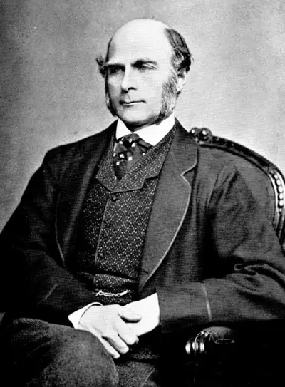
Moments are a set of statistical parameters to measure a distribution. Four moments are commonly used: 1. Mean 2. Variance: variance describes the scale of the distribution 3. Skewness 4. Kurtosis: Peakedness or flatness. kurtosis describes the spread of the distribution in a scale-independent manner

Francis Galton:

Inventor of eugenics

Discoverer of fingerprints!

Probability

Empirical probability: something observed in actual data. not generalized

Theoretical probability: truth that cannot be directly discovered

Mutually exclusive: the probability of each event happening is independent of another one happening

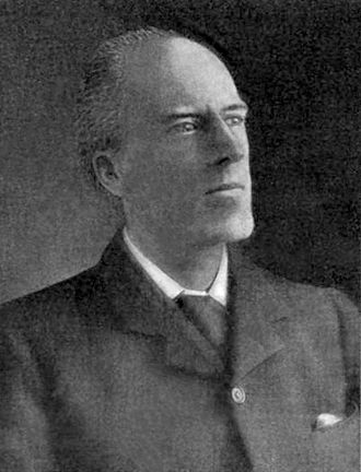
London born - in love with Karl Marx - studied Politics first - found out about regression to the mean

He became Galton's (Darwin's cousin) protégé!

💡

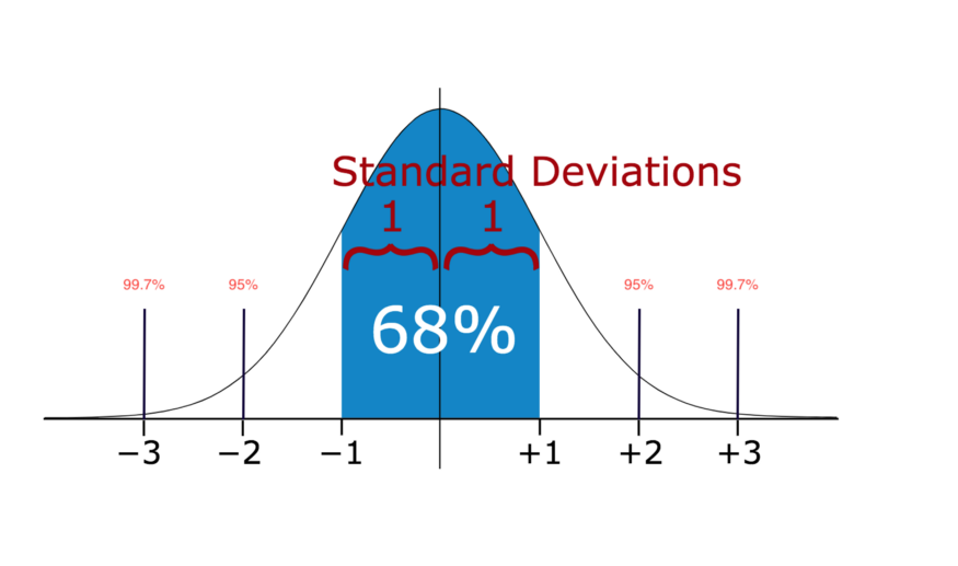
PDF If a random variable is continuous, then the probability can be calculated via probability density function, or PDF for short. The shape of the probability density function across the domain for a random variable is referred to as the probability distribution and common probability distributions have names, such as uniform, normal, exponential, and so on.

In statistics, If a data distribution is approximately normal then about 68% of the data values lie within one standard deviation of the mean and about 95% are within two standard deviations, and about 99.7% lie within three standard deviations

💡

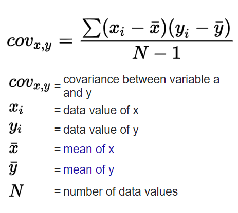
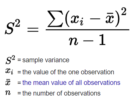
Cofounder (cofounding variable, extraneous determinant, etc.) Some variable that influences both dependent and independent variable that leads to a spurious association.

Covariance

Standard deviation and Variance

Variance is also distorted by outliers as it is calculated using our mean, and is sensible to large or small values. When the variance is low in one variable among many with similar scales, we can understand that this variable does not have much impact on our label.

Standard deviation → more sense : it's somehow the average amount we expect the records to differ from the average value.

The sample variance: a little smaller than the main variance

Correlation Coefficient (Pearson coefficient/r)

the covariance divided by the variance to bound the numbers.

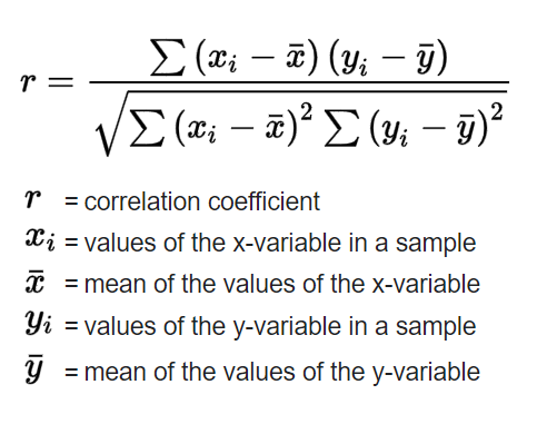
When two variables are correlated:

A causes B

B causes A

C causes A and B (C is a confounding factor)

Just coincidence

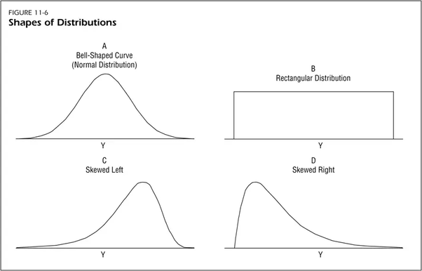
Skewness

The third moment

Right skewed: mode < median < mean

Left skewed: mode > median > mean

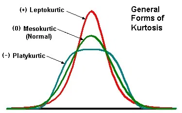
Kurtosis

Forth moment

how thick the ends are

Bias types:

Selection bias: you select only one part of the whole society\system\etc.

Undercoverage bias: We have samples from all groups but info from all groups are not balanced or adequate.

Survivor bias: We only view people\stocks\organizations that have survived. No data for those who got extinct!

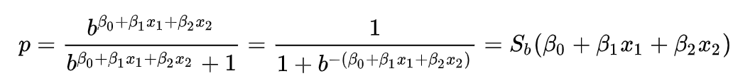
Logistic Regression

For understanding the logistic regression formula, we consider a logistic model that comes from a log of odds

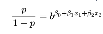
Odds of somethig

Is not its probability.

It's the ratio of something happening to something not happening.

Ex: we can win 5 games, we can loose 2, then the odds of our team winning is 2.5. Although the probability of my team winning is 0.71

💡

Log of adds (logits): its the log of odds. Why do we get the log? to make everything symmetrical. log(6) = - log(1/6)

Regression

coefficient of determination, denoted $R^2$

The proportion of the variation in Y being explained by the variance in x! a measure of how well observed outcomes are replicated by the model, based on the proportion of total variation of outcomes explained by the model.

${\bar {y}}$ is the mean of the observed data

$SSR = \sum (\hat{Y_i}-\overline{Y})^2$

$SST = SSM = \sum(Y_i - \overline{Y})^2$

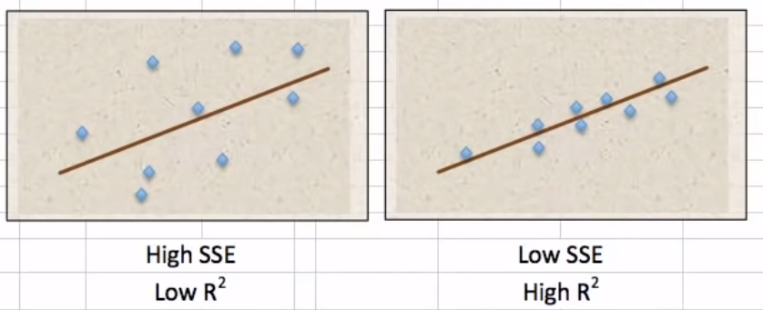
The denominator in R-squared is showing the variation in data as it is the deviation of each example from the mean of all examples. And the nominator is the distance of our predictions to the true values.

We can never know what beta null or one is but we can estimate them. The theory is that it exists.

Degrees of freedom

Degrees of freedom is determined by the number of observations and also the number of variables. the more data we have, the more freedom we have to move around our prediction line or plane. But the more variables there are the less freedom we have for defining the plane. So:

DegreesOfFreedom(df) = n-k-1

n: # of examples

k: # of variables

-1: for the label

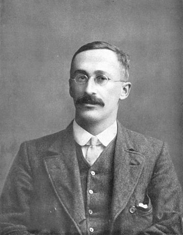
Criticized Pearson a lot!

Was a euginistic but not racist, I think.

Working on crops, he developed the ANOVA method.

He outlined hypotheses on natural selection and creatures population (e.g., the sexy son hypothesis!)

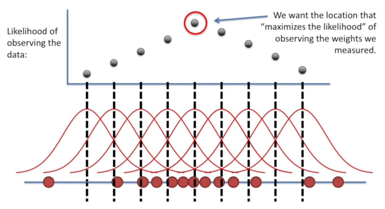
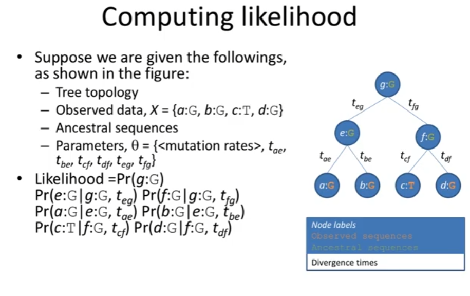
Maximum likelihood:

How likely it is for us to have this mean/center given this data

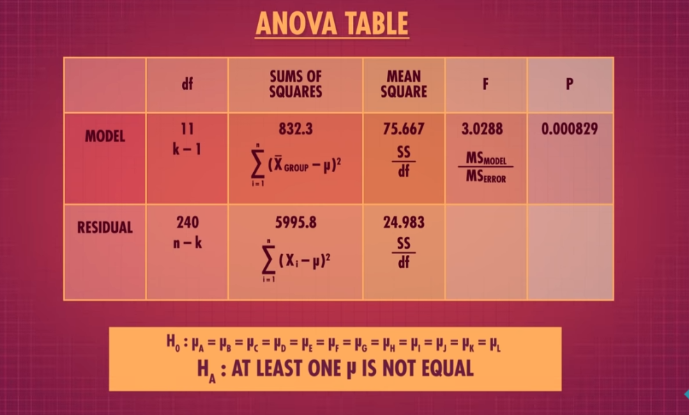
ANOVA

Analysis of variance. Extension of a t-test.

Assumptions: Distribution has a normal Distribution

Null hypothesis: There is no different\ relationship between two variables, means, etc.

result: p-value (how likely it is that these happened by accident and randomly) if it is less than our level of significance, we know that a statistically significant difference exist between groups or there is a statistically significant relationship between groups.

Adjusted R-squared

When we have low number of examples and two many variables our plane is defined by only those examples therefore we have a over-fitted plane.

To prevent this from effecting our model we adjust the R-squared.

The more variables, the less R-squared we will have.

\overline R^2 = 1 - (\frac {SSE}{SST} ).\frac{n-1}{n-k-1}

Hypothesis for regression

We say there is no relationship between X and Y unless we find enough evidence to reject this null hypothesis. When coeff is not null it is significant.

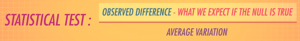
Test statistics

Does our score fit our null hypothesis well?

Z-score (The critical value)

How many standard errors we are away from the mean of the whole. We use it when we know the true population std. Like when we vaccinate people and know what percentage got sick so we calculated $p(1-p)$ and then got a sample of 600 and 400.

population. (when comparing two means from a samples and the mean of the whole population we're saying how many standard deviations we are away from the pop mean)

$Z_{group} = \frac{\overline{X}_{group} - Mean}{\frac{\sigma}{n}}$

with a critical value(threshold we identify whether or not the answer is significant, or whether or not we can reject the null)

T-student distribution

A posterior distribution (we know a little background of it- sample mean and variance).

T-test is a form of z-test. with large datasets we get the approximation of Z-test.

The author of its paper was interested in working on small samples from a larger population. It's a small sample size approximation of a normal distribution.

\frac{\overline{X}-\mu}{\frac{S}{\sqrt{n}}}

Effect Size: When using T-student and alpha make sure you actually take care of the size too as the std is being divided by the size of our sample. this may effect the t score and then we may get a small p-value!

Formula for groups:

$t-student = \frac{difference - 0}{Average variation}$

Chi squared

Pearson wanted more than a normal distribution!

He said if there are all from one normal distribution, we expect the mean and expected (n * p) to be from one group! (use critical value to calculate the probability of them being dependent)

It's only for categorical and nominal values!

With this we compare our model with the real and true sampled observations.

Relationship between two variables. For example, you could test the hypothesis that men and women are equally likely to vote "Democratic," "Republican," "Other" or "not at all."

Take continues variables and see how well we can test the fit of categorical variables.

test 🔗

$\chi^2$ Goodness of fitness

Many categories, one variable

💡

Check! Is the E for every category more than 5???

Formula:

$\chi^2 = \sum \frac{(O_i - Ei)^2}{E_i}$

Test of Independance

Checking if having one category in your features actually affects the variable we're checking!

Calculate the expected values and then compare them How to calculate the expected value??? Well, first of all how many said no? Then multiply this percentage with the total number of ravenclaws or hufflepuffs to see based on the distribution of yes and nos we have how many of ravenclaws or hufflepuffs we expect to have.

Test of Homogeneity

Whether two samples come from the same population

Interaction variables

Logit models (Logistic models)

F-Statistic and test

Fisher wanted to see the difference between different potato's weights based on the fertilizer they used!

He sampled from different fertilizers soil

calculated the difference between the mean of each group and the total mean,

squared it,

and divided it by fertilizer number - 1 (degrees of freedom of categories) →

got SSM, the error defined by the model/each group

Then calculated the difference between each value and all means

divided it by degrees of freedom which is the number of all samples -number of categories

got SSE

Then divided SSM by SSE → got F statistic

What is its p-value

Is there a difference? Yes? Reject the null of all being the same!!!

Types of data

Categorical and Quantitative

Quantitative

numbers with order and consistent spacing (an increase from 1 to 2 is the same increase we have when we go from 100 to 101) We turn quantitative into categorical by binning - especially when we have pre-existing bins (child, teenager, adult, old)

Categorical

no order or consistent spacing

vis: frequency table, relative frequency, contingency table (with totals)

He expounded the mathematics of extremes

Was a war war || survivor

Worked with Fisher

Experiments

Control group: no treatment, drug or change

Single blind study: the researcher knows about the change and purpose of study, but the volunteer does not

Matched pair experiments: on very similar people or groups.

Repeated Measures design: experiment with the same subject

In vitro experiments = test-tube experiments colloquially

Geometric distribution

P^s * (1-P)^{(1-s)}

Birthday paradox: unique birthdays given a number of people in one room.

Math revision

norm: magnitude of a vector Euclidean norm: l2 norm

💡

When to use L2? with large negative values. But when we want to calculate the norm of small non negative elements→ we use L1

Naïve Bayes🔗

The skewed distributions

Poisson distribution:

only has one parameter

Exponential distribution is one form of this

Trees

Singular value decomposition 🔗

The law of large numbers:

Perform the same task very frequently

basis of frequency-style thinking (deterministic way of thinking)

If you throw a fair, six-sided dice many times, the average of throwing it six times, the probability of each outcome, etc. will be clear (will get close to the expected value) after all those times.

Confounding variables = extraneous variables